Table of Contents
Spatial dis-aggregation CAPDIS module
Introduction
Environmental impact assessment of farm management decisions is often only possible in a spatial context, taking local conditions as land cover, climatic and soil conditions into account. Equally, farm management decisions depend to a larger extent on those local factors. Therefore, a CAPRI module has been developed that allows monitoring and ex-ante assessment of environmental impacts of agriculture at a 1×1 km spatial scale.
Purpose of disaggregation of CAPRI results
Update pending
A brief history of the CAPDIS module
Update pending
CAPRI-DynaSpat
HSU
Applications
Update pending
Link to DNDC-Europe
NitroEurope
European Nitrogen Assessment
IDEAg
CAPRI-RD
CAPDIS module – GUI basics
Files:
%curdir%/capdis.gms
%curdir%/capdis/capddis_relevantsets.gms
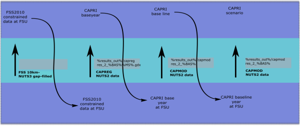
The distribution of crop shares, livestock numbers, yield and nitrogen flows is a sequential process of a number of sequential steps (CAPRI tasks). The distribution of land use and livestock numbers, yield and irrigation shares in each step is based on the results of the previous step which is used as priors.
A priori land use distribution (mode: LAPM): The first step uses statistical information available at the intersection of 10 km x 10 km grid cells and administrative units at the NUTS3 level (literature source to be pasted 
CAPREG disaggregation (mode: CAPREG): the a priori land use distribution is used as prior information to disaggregate statistical information for the CAPRI base year, currently the year 2012.
Timeseries disaggregation (mode: TIMESERIES): results from the CAPREG disaggregation are used as priors for the time series disaggregation.
Baseline and scenarios (mode: CAPMOD): results from the CAPREG disaggregation are used as priors for the ex-ante simulation results
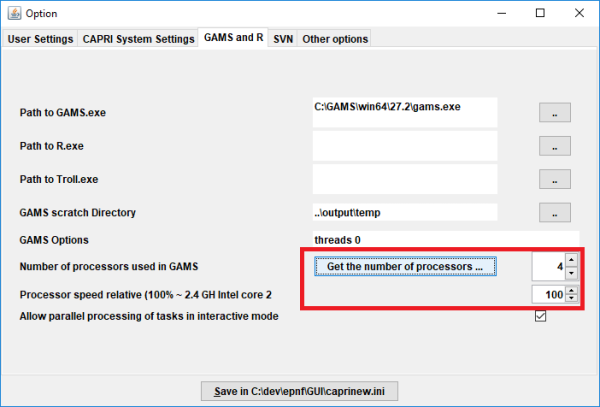
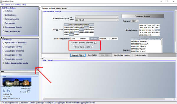
The disaggregation module works at the level of CAPRI NUTS2 regions, which are run in parallel mode. The number of parallel instances depends on the computing capacity (check CAPRI settings, tab ‘GAMS and R’, Number obtained from ‘Get the number of processors …’ or written into the combo box). To combine result files at regional level into country-level result files, a CAPRI task ‘Collect disaggregation results’ is available. This can be done for results of all other CAPRI disaggregation tasks. Optionally, a new country file can be generated (overwriting previous results) or an existing country file updated (overwriting only the data of the ‘new’ NUTS2 results). Also the NUTS2 files can be deleted.
Figure 42: Sequential disaggregation of land use
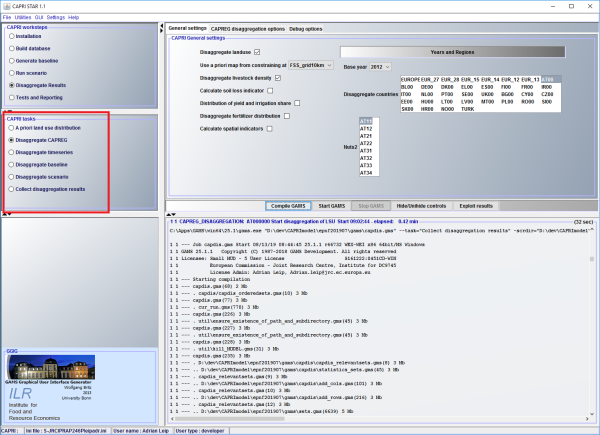
To activate CAPDIS (disaggregation module), select the CAPRI workstep “Disaggregate Results”. Then select one of the following CAPRI tasks: A priori land use distribution, Disaggregate CAPREG, Disaggregate timeseries, Disaggregate baseline, Disaggregate scenario, or Collect disaggregation results. All tasks can run in one go, or in separate simulations, if result files of the previous variable are available (e.g. land use already disaggregated for the disaggregation of livestock).
Farm Structure Units – FSU
Files:
%datdir%/capdishsu/s_fsu_srnuts2.gdx
%datdir%/capdishsu/fsunogo.gms
%datdir%/capdishsu/m_grid10n2.gms
%datdir%/capdishsu/p_fsu_grid10n2.gdx
%datdir%/capdishsu/p_fsu_srnuts2.gdx
%datdir%/capdishsu/p_fsu_area.gdx
%datdir%/capdishsu/p_fss2010.gdx
Delineation
Update pending
Administrative units
Inspire grid
Soil mapping units
NOGO and Forest units (Corine)
Data preparation
Update pending
Determination of the centre
Corine Shares
DEM
PESETA
EMEP
Disaggregation of crop Areas
Files:
%curdir%/capdis/disyield.gms
%curdir%/capdis/disyield_sets.gms
%curdir%/capdis/m_hpdCropSpat.gms
%datdir%/capdishsu/pesetagrid_fractionfsu.gdx
%datdir%/capdishsu/irriShare2000fsu.gdx
The principle of the distribution of crop areas is based on few constraints only: full exhaustion of available ares for each spatial unit, vertical consistency, and primacy of land stability.
Vertical consistency means that the sum of each land use type over all spatial units recovers available land use at the higher spatial level. As available information are not (necessarily) geo-referenced, the allocation of a given statistical information to a spatial unit is associated with uncertainty. For example, a farmer with the residence in region A can have land also in regions B and C, but will declare them together, and they will be allocated to her residence (region A). Accordingly, there is some blurring in particular at boundaries and this is accounted for in the methodology: also at the high disaggregation level, the land uses are principally to be interpreted as ‘Land owned by a farmer with residence in this spatial unit’.
Primacy of land stability means that if there is no indication (i. e. new observation, policy restricting previous land distributions, …) it is more likely that the spatial pattern remains similar to the previous (prior) pattern. Therefore, once a likely distribution of land and livestock has been determined on the basis of high-resolution FSS statistics, the model tries to stay as close as possible to this distribution. This is achieved with penalty factors that are activated as soon as the estimated land use area deviated from the prior values, assigning a higher penalty for deviations of permanent crops and forests, and very high penalties of a land use is estimated in a spatial unit where it didn’t exist in the prior’s data base.
The disaggregation model m_hpdCropSpat is described in Section Simulation model m_hpdCropSpat.Section Data sets describes the required input data, and Section Data preparation describes the preparation of the input data for their use in hpdCropSpat.
Simulation model m_hpdCropSpat
Equation 1 RULEVL_
     The levels assigend to the FSUs must recover the given NUTS II area
     both NUTS2 level and FSU level in 1000 ha
     rur = grid cell in mode LAPM, rur = NUTS2 in all other modes
RULEVL_(rur,curact) ..
SUM(regmap(rur,cur%spatunit%),v_levlCon(rur,cur%spatunit%,curact))
=E= p_nutsLevl(rur,curact);
\begin{equation} A_{c^*,r}=\sum_h\{a_{c^*,h}\} \end{equation}
\(a_{c^*,h}\) = Area [parameter, km2] cultivated with crop c or covered by ‘other land’ use excluding forest in spatial unit h
\(A_{c^*,h}\) = Area [parameter, km2] cultivated with crop c or covered by ‘other land’ use excluding forest in region r
Equation 2 ADDUPGRID_
Due to several reasons it could be impossible to distribute all agricultural area under the given constraints of total available area in the spatial units (net of the area of ‘nogo’ units and forest area). In order to enable a feasible solution, an error term is introduced that allows the units to slightly shrink or grow. The reason:
- Statistical data are not (necessarily) geo-referenced; i.e. an area of crops (or a livestock) might be assigned to one unit/grid cell because this is where the farm is registered rather than the physical location of crop/livestock
- Uncertainties in the data
- Inconsistencies of data sources (i.e. FSS agricultural statistics, Corine Land Cover data, CAPRI regional statistics)
- – The FSU area must be exhausted, but the variable v_%spatunit%SizeChg
allows some flexibility if needed.
ADDUPGRID_(rur,cur%spatunit%) $ p_levlunit(rur,cur%spatunit%,"area") ..
SUM(curact,v_levlCon(rur,cur%spatunit%,curact))
=E=
v_%spatunit%SizeChg(rur,cur%spatunit%)*p_levlunit(rur,cur%spatunit%,"area");
\begin{equation} a_h⋅\epsilon_{a,h}=\sum_{c^*}\{a_{c^*,h}\} \end{equation}
\(a_h\) = Area [parameter, km2] of spatial unit h
\(a_{c^*,h}\) =Area [parameter, km2] cultivated with crop c or covered by ‘other land’ use excluding forest in spatial unit h
\(\epsilon_{a,h}\) = Error term, allowing a spatial unit to shrink or grow slightly in order to enable a feasible disaggregation of statistical data.
Equation 3 PDF_
The most likely solution is obtained with the ‘Highest Posterior Density’ method. A penalty function calculates deviations from prior information, applying uncertainties
- A random re-allocation of crops should be avoided. Therefore, a penalty is given with increasing deviation from the prior distribution to ensure stability in the time series
- In particular the ‘appearance’ of crops in spatial units where they have not been observed in the prior data should be restricted (disagg(“penelizenewcrops”))
- The error term for the area of the spatial units should be kept at a minimum (disagg(“penalizesizechange”))
PDF_ ..
# Scale density value a good couple of magnitudes for numerical reasons.
v_hpd
*[SUM((curact,regmap(rur,cur%spatunit%)) $ p_levlStde(cur%spatunit%,curact),
p_levlunit(rur,cur%spatunit%,"area"))
 +SUM(regmap(rur,cur%spatunit%) $(v_%spatunit%SizeChg.LO(rur,cur%spatunit%) NE
v_%spatunit%SizeChg.UP(rur,cur%spatunit%)),
    p_levlunit(rur,cur%spatunit%,"area"))
 ]
=E=
# hsu area-weighted mean square of the deviation from prior mean area, scaled by its stdev
(SUM((regmap(rur,cur%spatunit%),curact),p_levlunit(rur,cur%spatunit%,"area")
       * SQR( (v_levlCon(rur,cur%spatunit%,curact)-p_levlunit(rur,cur%spatunit%,curact))
               *(                  1 $      p_levlunit(rur,cur%spatunit%,curact)
                  + disagg("penalizenewcrops") $ (not p_levlunit(rur,cur%spatunit%,curact)))
               /max(1e-3,
                         $$ifi     %MODE%==LAPM p_levlStde(cur%spatunit%,curact)
                         $$ifi NOT %MODE%==LAPM 1
                   )
             ) \\
    )/SUM((regmap(rur,cur%spatunit%),curact)  \\
$p_levlStde(cur%spatunit%,curact),p_levlunit(rur,cur%spatunit%,"area")) \\
)$sum((regmap(rur,cur%spatunit%),curact),p_levlStde(cur%spatunit%,curact)) \\
# penalty for deviation from hsu area \\
+(SUM(regmap(rur,cur%spatunit%),  \\
disagg("penalizesizechange")*p_levlunit(rur,cur%spatunit%,"area")*SQR((v_%spatunit%SizeChg(rur,cur%spatunit%)-1))) \\
 /SUM(regmap(rur,cur%spatunit%), p_levlunit(rur,cur%spatunit%,"area")) \\
 )$SUM(regmap(rur,cur%spatunit%),p_levlunit(rur,cur%spatunit%,"area")) \\
; \\
Model parameters
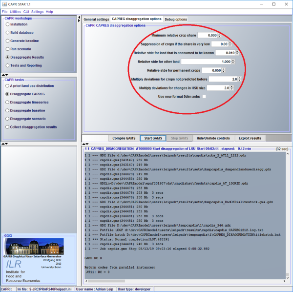
Some model parameters can be set by the user through the CAPRI GUI.
They are collected in the parameter ‘disagg’.
set disaggcontrol /
mincropshare "Minimum allowed cropshare per HSU"
relcropshare "Defines heterogeneity of crop shares for a crop per HSU"
relstdefix   "Relative standard deviation, predefined if land needs 'to be fixed'"
relstdeperm  "Relative standard deviation, predefined for permanent crops"
relstdeothe  "Relative standard deviation, predefined for other land (large to avoid that other land pushes agriland around)"
penalizenewcrops   "multiply deviations for crops predicted where they haven't been before"
penalizesizechange "multiply deviations for total HSU unit size"
* --- scalars controlling livestock disaggregation
weightRUMIfodduaar "Weighting between fodds and uaar to distribute initial RUMI numbers"
weightMONOcereuaar "Weighting between cereals and uaar to distribute initial NRUMI numbers"
minLSUdens          "Minimum density for LSU allowed to not have them everywhere...     "
# managing crop residues
minmcactSurs   #Miniumum surplus as compared to average over all crops
maxmcactSurs   #Maxiumum surplus as compared to average over all crops
rangemcactSurs #Range of sursoi (max/average) below which the high sursoi are not reduced
/;
- Stability of forests – disagg(“relstdefix”)
Forests cannot easily be ‘displaced’ and are likely to remain rooted as given in the land cover data sets. So far, estimations of changes of forest areas at the regional level are not included in the disaggregation procedure.
The default value used for disagg(“relstdefix”) = 0.01
The lower the value the higher becomes the penalty if the estimates are deviating from the priors.
- Stability of permanent crops disagg(“relstdeperm”)
Permanent crops are long-term investments and require time to grow. Displacement of permanent crops is slow.
The default value used for disagg(“relstdeperm”) = 0.05.
- Coefficient of variation for ‘other land uses’ disagg(“relstdeothe”)
‘Other’ area is a lump of all non-agricultural areas. We consider this area as relatively flexible.
The default value used for disagg(“relstdeothe”) = 1.
- Penalization for new crops in spatial units disagg(“penalizenewcrops”)
New crops ‘appearing’ in spatial units, if they have not been in the priors data set, are penalized. The penalization factor is a multiplicator of the squared deviation from the prior. Thus, the higher the factor the higher becomes the penalty.
The default values used for disagg(“penalizenewcrops ”)=2.0;
- Penalization of area changes of spatial units disagg(“penalizesizechange”)
The default values used for disagg(“penalizesizechange”)=2.0;
- Minimum crop share allowed in the spatial unit disagg(“mincropshare”)
The minimum crop share which is allowed in the spatial unit χ_(min ) is used to calculate the lowest allowed crop share, in combination with the minimum relative crop share defining the level of spatial heterogeneity for a crop. See section 7.4.3.5 
\(χ_{min}\) can be set through the CAPRI GUI (tab CAPREG disaggregation options – “Suppression of crops if the share is very low”)
By default, \(χ_{min}\)is set to zero.
- Minimum relative crop share disagg(“relcropshare”)
The minimum relative crop share defining the level of spatial heterogeneity for a \(χ_{rel}\) is used to calculate the lowest allowed crop share, in combination with the m crop minimum crop share which is allowed in the spatial unit (see section 7.4.3.5 
\(χ_{rel}\) can be set through the CAPRI GUI (tab CAPREG disaggregation options – “Minimum relative crop share”)
By default, \(χ_{rel}\) is set to zero.
Defining bounds for the land use distribution model
Bounds for size changes of the total area of the spatial units
v_%spatunit%SizeChg.L (rur,cur%spatunit%) $p_temp3dim(rur,cur%spatunit%,"crops")= 1;
v_%spatunit%SizeChg.UP(rur,cur%spatunit%) $p_temp3dim(rur,cur%spatunit%,"crops")= 1.1;
v_%spatunit%SizeChg.LO(rur,cur%spatunit%) $p_temp3dim(rur,cur%spatunit%,"crops")= 0.9;
v_%spatunit%SizeChg.UP(rur,cur%spatunit%)
$(p_nutslevl(rur,"AREAcorr") and p_temp3dim(rur,cur%spatunit%,"crops"))= 2.0;
v_%spatunit%SizeChg.LO(rur,cur%spatunit%)
$(p_nutslevl(rur,"AREAcorr") and p_temp3dim(rur,cur%spatunit%,"crops"))= 0.5;
$$ifi %MODE%=="LAPM" v_%spatunit%SizeChg.UP(rur,cur%spatunit%) $p_temp3dim(rur,cur%spatunit%,"crops")=
max(1.1,p_nutslevl(rur,"AREAcorr"));
$$ifi %MODE%=="LAPM" v_%spatunit%SizeChg.LO(rur,cur%spatunit%) $p_temp3dim(rur,cur%spatunit%,"crops")=
1/max(1.1,p_nutslevl(rur,"AREAcorr"));
To enable the solver to find feasible solutions even in difficult situations, it is possible to expand or shrink the total area of the spatial units. This is in consistence with the definition of the data compiled by the statistical offices which link the area to residence to the farmer rather than to the geographic location of each field.
Generally, we limit this area-change to plus/minus 10% of the original size.
In cases where inconsistencies between data sets have already been identified (see 0) a higher degree of flexibility is allowed (factor 2) as it is not known in which spatial unit the inconsistency originated.
Only in the task ‘A priori land use distribution’ the degree of flexibility is calculated as a function of the correction that had to be applied to the regional area.
The bounds for the area-size change are hard-coded and can not be changed by the user.
Setting standard deviations
Data do not come with any level of uncertainty attached, and there is no a priori information on what spatial distribution is more likely than any other.
Therefore, the uncertainty in the estimates is ‘guessed’ based on crop groups.
Other options tested (all standard deviations equal or scaling prior estimates to a plausible range) are currently not used. The standard deviations are only set at the first task. In subsequent tasks, the standard deviations of the priors are used and ‘gap-filled’ if necessary.
$set changelapmstdev bygroups
$iftheni.std %changelapmstdev%=="scalestdevs"
$elseifi.std %changelapmstdev%=="allone"
$elseifi.std %changelapmstdev%=="bygroups"
    p_levlstde(cur%spatunit%, %croptp%)
*        $ p_levlstde(cur%spatunit%, %croptp%)
      = 0.5;
    p_levlstde(cur%spatunit%, %croptp%)
*        $ p_levlstde(cur%spatunit%, %croptp%)
      = 0.001 $sum(fssact2groups(%croptp%, "FORE"), 1)
      + 0.50  $sum(fssact2groups(%croptp%, "CERE"), 1)  # Cereals incl those likely in rotation: Assumptions market oriented might change relatively quickly if price is correct
      + 0.25  $sum(fssact2groups(%croptp%, "FODD"), 1)  # Fodder crops: roof, ofar, lgras. Assumption: link to livestock which do not shift around so quickly
      + 0.25  $sum(fssact2groups(%croptp%, "OILS"), 1)  # Oil crops: rape, sunflower, soya. Assumption: relatively sticky
      + 0.15  $sum(fssact2groups(%croptp%, "VEGE"), 1)  # Vegetables: flower, pulses, potatoes, sugar beet, ... but also tobacco, text etc. Assumption: require often infrastructure (greenhouse) so longer investments required
      + 0.05  $sum(fssact2groups(%croptp%, "TREE"), 1)  # Permanent crops: olives, nurseries, fruit and nuts trees, vinyards. There are permanent
      + 0.05  $sum(fssact2groups(%croptp%, "PERM"), 1)  # Permanent crops: olives, nurseries, fruit and nuts trees, vinyards. There are permanent
      + 0.80  $sum(fssact2groups(%croptp%, "REST"), 1)  # Assumptions: can be easily pushed around
      ;
Data sets
Update pending
FSS 2010 data at nested grid levels
FSS 2010 data, gap-filled at 10km-NUTS3 overlay
Forest map
Data preparation
Re-mapping from FSS crops to CAPRI crops
# Convert to CAPRI activities (posteact)
#As grids and NUTS are not always consistent - use the grid-HSUs to fill with crops
p_hsufraction(curgrid,%spatunit%_all)=p_hsu_grid10n23(%spatunit%_all,curgrid,"fracHSU");
grid10n23_hsu(curgrid,%spatunit%_all)$p_hsufraction(curgrid,%spatunit%_all)=yes;
cur%spatunit%(%spatunit%_all)=yes$sum(grid10n23_hsu(curgrid,%spatunit%_all),1);
Intersecting FSS 2010 10km x NUTS3 to FSU
The land use distribution model works at the spatial intersection of the prior and posterior spatial units. Historically (when CAPDIS was based on HSU) this intersection was an area determined by the fraction of the HSU that lies within different FSS-admin grid cells. This fraction \(f_{hg}\in[0,1]\).
However after the update to the FSU, each spatial unit was fully in one FSS-admin grid cell only, thus \(f_{hg}\in\{0,1\}\). The following text is therefore relevant only if CAPDIS is run with ‘old’ HSU.
# Work on the intersection between grid and HSU (Line 585 ff)
p_levlunit(%region%,cur%spatunit%,"AREA")
=p_hsufraction(%region%,cur%spatunit%)*p_hsu(cur%spatunit%,"area");
" Work on intersection of HSU and grid for crops"' '" "'
# Distribute crops over intersected units –and scale to total area (should be already but not always is...)
p_levlunit(%region%,cur%spatunit%,%croptp%)
=p_hsufraction(%region%,cur%spatunit%)*p_levlmean(cur%spatunit%,%croptp%);
# Scale all areas such that the sum becomes the AREA of the unit (in case the HSU had to be split)
#    - if LAPM predictions are consistent with total area
p_temp3dim(%region%,cur%spatunit%,"allarea")
=sum(%croptp%$(not sameas(%croptp%,"FORE")),p_levlunit(%region%,cur%spatunit%,%croptp%));
p_levlunit(%region%,cur%spatunit%,%croptp%)
$(p_temp3dim(%region%,cur%spatunit%,"allarea") and not sameas(%croptp%,"FORE"))
=p_levlunit(%region%,cur%spatunit%,%croptp%)*(p_levlunit(%region%,cur%spatunit%,"AREA")-
	p_levlunit(%region%,cur%spatunit%,"FORE"))
	/p_temp3dim(%region%,cur%spatunit%,"allarea");
In order to ensure consistency of total area between the prior and the posterior data sets, all data are re-mapped into their intersection. This is achieved with the fraction of the spatial units of one layer that is part of a unit of the second spatial layer:
\begin{equation} a_{hg}=\sum_{h,g}\{a_h\cdot f_{hg} \} \end{equation}
\(a_{hg}\) = Area [parameter, km2] of unit u intersecting spatial unit h and grid cell g.
\(a_h\) = Area [parameter, km2] of spatial unit h
\(f_{hg}\) = Fraction of spatial unit h, which is covered by grid cell g
Cultivated crop areas are re-mapped to the intersecting units proportionally to the area fraction, assuming homogeneous distribution of each crop within each spatial unit h.
The LAPM predictions are not constrained to exhaust the total available area. However, this is a required characteristic in CAPRI. Therefore, the land use areas (crops, forest land and ‘other’ area) are scaled so that their sum matches the total available area. As forest areas are obtained from a data set, which is assumed to be of high precision, forest areas are excluded from scaling.
\begin{equation} a_{c^o,hg}=\sum_{h,g} \left\{ a_{c,h} \cdot f_{hg} \cdot \frac{a_{hg} - a_{forest,hg}}{\sum_{c^{o^\prime}} a_{c^{o^\prime}}} \right\}, \end{equation}
\(c^*\) = Land use. \(c^*\in\{c,other \; land\}\)
\(a_{c^o,hg}\) = Area [parameter, km2] cultivated with crop c or covered by ‘other land’ use excluding forest in unit u intersecting spatial unit h and grid cell g.
\(a_{c^o,h}\) = Area [parameter, km2] cultivated with crop c or covered by ‘other land’ use excluding forest in spatial unit h
\(f_{hg}\) = Fraction of spatial unit h, which is covered by grid cell g
Note that this re-mapping is done in each step, however it affects only the step ‘A priori land use distribution’ which is constrained by data for the intersections of the FSS-10km grid cells with NUTS3 regions. These units are not aligned with the spatial units (HSU) for two reasons:
- HSU are aligned with a regular grid of 0.25° x 0.25° but not to a grid of 10 km x 10 km
- Even though HSU are aligned with a NUTS3 administrative region layer, changes in the definition of NUTS3 regions over time create shifts in the boundaries
In all other steps, the constraining data set is taken from CAPRI NUTS2 regions to which all spatial units are nested to and \(f_{hr}=1\forall h,r\).
The same holds if disaggregation is done into the FSU units, which are part of exactly one FSS grid cell.
Dealing with FSS grid cells with too much crops
Line 613ff
p_temp3dim(%region%,"AREA","<0")$(p_nutslevl(%region%,"AREA") and (p_nutslevl(%region%,"OTHER")<0))
=(p_nutslevl(%region%,"CROPS")+p_nutslevl(%region%,"FORE"))/p_nutslevl(%region%,"AREA");
p_nutslevl(%region%,"AREAcorr")=p_temp3dim(%region%,"AREA","<0");
# Rescale total and crop area of units if the total area in the %region% had to be changed.
p_levlunit(%region%,cur%spatunit%,"AREA")$(p_temp3dim(%region%,"AREA","<0"))
=p_levlunit(%region%,cur%spatunit%,"AREA")*p_temp3dim(%region%,"AREA","<0");
p_levlunit(%region%,cur%spatunit%,"OTHER")$(not p_temp3dim(%region%,"AREA","<0"))
=max(0,p_levlunit(%region%,cur%spatunit%,"AREA")-
		sum(%croptp%,p_levlunit(%region%,cur%spatunit%,%croptp%)));
Farm structure surveys collect data on crop areas and allocate them to the geographic location where the farmer resides. Therefore, it is not excluded that a spatial unit (grid cell) has more crop area than the cell is large. It is not possible to ‘correct’ those allocations.
CAPRI works with an area-consistent approach, thus the total area available must be exactly matching the sum of the areas used for different purposes. As a re-allocation of ‘surplus’ crop areas is not possible, we inflate the area of spatial units h so that all forest and crop areas can be accommodated. The area of ‘other’ land uses is adapted to ensure coherence.
\begin{equation} a_{hg} \leftarrow a_{hg} \cdot \frac{a_{g,forest} + \sum_c a_{g,c}}{a_g} \end{equation}
\begin{equation} a_{hg, other} = a_{hg} - a_{hg,forest} - \sum_c a_{hg,c} \end{equation}
Note that this ‘manipulation’ of the data is needed to avoid any potential infeasibilities in the land use disaggregation model maintaining the relevant information from the different data sets:
- The total crop areas data collected in the FSS
- The heterogeneity of crop areas (‘suitability’) as modelled with the LAPModel. This concerns both the spatial heterogeneity within a region across spatial units, as well as the relative abundance of different crops in a single spatial unit.
Adding previously unobserved crops
It might well be that crops occur in a grid cell or region which were not predicted or which had not been observed ‘before’ (e.g. when moving from ex-post to ex-ante simulation). In this case prior estimates of the distribution need to be developed.
This is done on the basis of ‘similarity’ assuming that similar crops have similar preferences for natural conditions (or available infrastructure) and a similar spatial heterogeneity.
This ‘gap-filling’ is done in three hierarchical steps:
1. Average crop area of similar crops in the same spatial unit as defined in the set mactgroups:
set mactgroups(sgroups,*) "Groups with similar crops - LAPM activities" /
  CERE.(BARL,SWHE,DWHE,LMAIZ,OATS,RYEM,OCER,PARI)
  VEGE.(TOMA,OVEG,SUGB,POTA,PULS,FLOW)
  FODD.(ROOF,OFAR,LGRAS)
  OILS.(SOYA,LRAPE,SUNF)
  FORE.(FORE)
  TREE.(APPL,CITR,OFRU,NURS,NUTS,LOLIV,LVINY)/;
2. If there are no ‘similar’ crops in the region or grid cell, the average area of all available crops is used.
3. If there is still no prediction of the in the spatial unit, the same crop area is given to the prior estimates in all spatial units in the region/grid cell.
Checking availability of standard deviations
May become obsolete for the CAPDIS modules of the CAPRI stable release versions following STAR 2.4
The LAPModel provides not only prediction for crop shares for each HSU, but at the same time also an estimate for the standard deviation of each estimate. These standard deviations are ‘carried’ on throughout the CAPRI disaggregation steps.
The procedures described above however made evident that some crops might appear in spatial units where they have not been observed before; obviously, an estimate of the standard deviation must be provided as well.
If the crops have been observed in other spatial units of the region or grid, the maximum relative standard deviation is used. If the crop has not been observed in the whole region or grid, the maximum standard deviation over all observed crops is used. Still missing standard deviations are assumed to be 100%.
Standard deviation for ‘other land uses’ are also set to a default of 100%, but can be modified by the user (through the CAPRI GUI).
Preparation for specific applications
Lines 690ff
p_temp3dim(%region%,"loshare",%croptp%)$ p_nutslevl(%region%,%croptp%)
= max(disagg("mincropshare"),p_temp3dim(%region%,"share",%croptp%)*disagg("relcropshare"));
p_levlunit(%region%,cur%spatunit%,%croptp%)
$((p_levlunit(%region%,cur%spatunit%,%croptp%)/sum(%croptp%1,p_levlunit(%region%,cur%spatunit%,%croptp%1))
<p_temp3dim(%region%,"loshare",%croptp%)) and not (sameas(%croptp%,"other")))
=0;
For some applications, the focus is on the analysis of dominant crops in each spatial unit, for example, when linking the result of the disaggregation with process-based crop models. This is done on the basis of two parameters:
\begin{equation} a_{hc}= 0 \leftarrow \frac {a_{h,c}} {\sum_{c^{\prime}}a_{h,c^\prime}} \lt max \left[ χ_{min},\frac{a_{r,c}}{\sum_{c^\prime}a_{r,c^\prime} } \cdot χ_{rel} \right] \end{equation}
\(χ_{min}\) = Minimum crop share allowed in the spatial unit
\(χ_{rel}\) = Minimum relative crop share – defines heterogeneity of crop shares for a crop in a spatial unit
Downscaling of Livestock numbers
Files:
%curdir%/capdis/dislivestock.gms
%datdir%/capdishsu/corine2018classes.gms
%datdir%/capdishsu/s_fracGraz.gms
%datdir%/capdishsu/p_fracGraz.csv
%datdir%/capdishsu/p_grazsharesCorine.gms
%datdir%/capdishsu/p_fsuCorineArea.gdx
A different approach is used for the distribution of FSS livestock numbers and for the distribution of CAPRI regional data. This is because livestock require some investment/infrastructure that is not easily given up. Also, if feed is more difficult to grow due to a dry or heat spell (e.g. as observed in 2018 in several countries), feed will be purchased from the market or animal numbers.
For livestock there will also apply the principle of the ‘Primacy of stability’ already described for the distribution of crop areas.
Animal types are distributed proportionally to their shares in different animal classes:
- Grazing cattle
- Grazing sheep and goats
- Non-grazing ruminants (cattle, sheep and goats)
- Non-grazing monogastric animals (pig and poultry)
Distribution of FSS livestock numbers
We use shares of grazing animals from the national submissions of greenhouse gas inventories to the UNFCCC. These shares are calculated from the quantity of manure N managed in various manure management systems, and the quantity of manure N deposited on ‘pasture, range and paddock’ (Table 3.B(b) of the UNFCCC-Common Reporting Format, CRF, tables).
The distribution of grazing livestock from the FSS grid cells to the FSU is done using areas of various Corine classes as a proxy. This is because grazing can occur also on non-grassland, such as on commune land (outside of the CAPRI UAAR) and mixed land cover classes (agro-forestry, non-agriculural land (shrubland, etc.).
Based on expert information obtained from the EEA (Jan-Erik Petersen, personal communication), the sum of the following Corine class shares is calculated:
# Corine classes to be used to calculate grazing shares and areas
#
# Source: EEA (Jan-Erik Petersen) in email from 19/07/2019.
# See kipinca-CLC classes + grazing_draft_+JRC questions_rev 23-07-19.docx
# Animal types distinguished: DairyCattle, NonDairyCattle, SheepGoats
parameter p_CorineShares(*, *, *) 'Shares of CLC area used to distribute grazing animals';
table p_CorineShares
       DairyCattle  NonDairyCattle SheepGoats
all.211           25             25          10
all.223            0              0          25
all.231          100            100         100
all.242           25             25          25
all.243           50             50          50
all.244           50             50          50
all.321          100            100         100
all.322           25             25          50
all.323           25             25          50
all.324            0              0           0
all.333           25             25          25
all.411           50             50          50
all.412            0              0          25
all.421           50             50          50
;
For classes 322 ('Moors_and_heathland') and 324 ('Transitional_woodland-shrub') a differentiation by countries is done.
We assume that for grazing animals, the density of \(v_{lgr}\) [LU ha-1] is constant within each FSS-admin grid cell and the number of livestock depends on the relevant Corine area.
\begin{equation} ν_{lgr,h}= N_{l,r} \cdot χ_{graz,lgr,r}\cdot A_{lcl,lgr,r} \end{equation}
\begin{equation} n_{lgr,h}= ν_{lgr,h} \cdot a_{lcl,lgr,h} \end{equation}
\(ν_{lgr,h}\) = Livestock density [parameter, LU ha-1] for animals in livestock group lgr in spatial unit h
\(N_{l,r}\) = Number of livestock [parameter, LU] of animal type l in region r
\(n_{lgr,h}\) = Number of livestock [parameter, LU] of animals in livestock group lgr in region r
\(χ_{graz,lgr,r}\) = Share of grazing animals [parameter, dimensionless] of animals in livestock group lrg in region r
\(A_{lcl,lgr,r}, a_{lcl,lgr,h}\) = Area [parameter, 1000 ha] of Corine Land Cover Classes lcl that are assumed to be available for grazing animals in livestock group lgr in spatial unit h.
Distribution of CAPRI livestock numbers
If livestock numbers change at the regional level if compared to the prior data, we assume that this has no influence on the spatial distribution of the animals. Instead, the livestock number in each spatial unit is multiplied with the regional relative change.
\begin{equation} n_{l,h}= \hat{n}_{lgr,h} \cdot \frac {N_{l,r}}{\hat{N}_{l,r}} \end{equation}
\(n_{l,h}\) Number of livestock [parameter, LU] of animal type l in spatial unit h.
\(\hat{n}_{l,h}\) Number of livestock [parameter, LU] of animal type l in spatial unit h in the prior data set
\(N_{l,r}\) Number of livestock [parameter, LU] of animal type l in region r
\(\hat{N}_{lhr}\) Number of livestock [parameter, LU] of animal type l in spatial unit h in the prior data set
Disaggregation of Nitrogen Input
Nitrogen input to fields needs to be distributed over the spatial units in a region where the crop is cultivated. For each crop, the regional nitrogen balance is given with total N inputs per N input type, an N outputs or losses per output and loss type.
We base the distribution model on a generic crop-fertilizer-response curve. Such curves have the characteristics that are desirable for the disaggregation of nitrogen input:
- higher N input leads to higher yields;
- with increasing levels of N input the yield increment decreases;
- the N ‘uptake’ is always less of N input;
- saturation, i.e. attaining about 80-90% of the maximum yield at about 100-200 kg N ha-1 yr-1
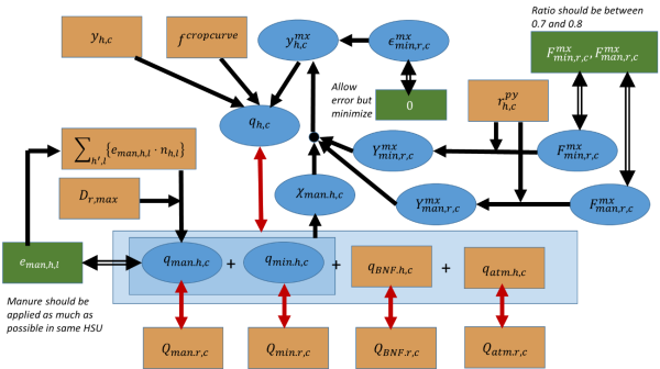
Such crop response curves ‘work’ with a maximum yield which are approached at high levels of N input. These maximum yield values are unknown. Figure below gives an overview of the approach indicating parameters, variables, and optimization rules.
Figure 43: Schematic overview of the Nitrogen disaggregation model

Crop response curve
Different crop response curves are proposed (Bodirsky and Müller, 2014; Godard et al., 2008). We base our response curve on the proposal of (Godard et al., 2008) in particular for the ‘saturation’ velocity1).
\begin{align} \begin{split} &\text{Crop growth model (Godard et al., 2008)} \\ &Y_{r,c} = Y_{r,c}^{mx}-(Y_{r,c}^{mx}-Y_{r,c}^{mn}) \cdot exp\{-f^{cropcurve}\cdot Q_{r,c}\} \end{split} \end{align}
\begin{align} \begin{split} &\text{Crop growth model (Godard et al., 2008) without ‘minimum yield’} \\ &Y_{r,c} = Y_{r,c}^{mx}-(1 - exp\{-f^{cropcurve}\cdot Q_{r,c}\}) \cdot @ Y_{r,c}^{mn} = 0 \end{split} \end{align}
\(Y_{r,c}\) = Yield [parameter, kg N ha-1 yr-1] for crop c in region r.
\(Y_{r,c}^{mx}\) = Maximum yield [parameter, kg N ha-1 yr-1] according to the crop response curve (Godard et al., 2008) for crop c in region r.
\(Y_{r,c}^{mn}\) = Minimum yield [parameter, kg N ha-1 yr-1] according to the crop response curve (Godard et al., 2008) for crop c in region r. This parameter is set to zero in our model.
\(f^{cropcurve}\) = Scaling factor [parameter, dimensionless] used in the crop response curve (Godard et al., 2008). We use a uniform value of \(f^{cropcurve}=0.008\).
\(Q_{r,c}\) = Total N input [parameter, kg N ha-1 yr-1] for region r and crop c.
Crop growth scaling factor
We use a constant factor \(f^{cropcurve}\) for all regions/spatial units and crops in order to not leave too many degrees of freedom. However, if infeasibilities occur, ‘opening’ this factor to differ between crop types could be a first test. However, the range of possible values for the crop growth scaling factor is narrow:
- For \(f^{cropcurve}>0.010\) a N uptake is larger than N input until an application rate of more than 100 kg N ha-1 yr-1. For a value of 0.010 this is the case for an application rate of about 100 kg N ha-1 yr-1
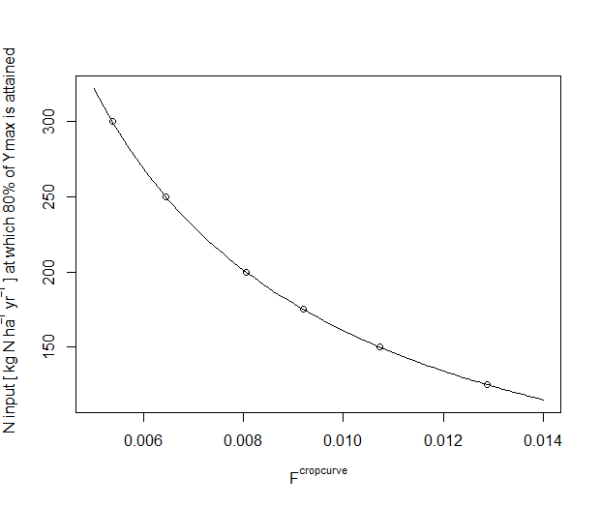
- For \(f^{cropcurve}<0.008\) the N input rate at which a yield of 80% of the maximum yield is attained is very high. For a value of 0.0064 this happens at Q=250 kg N ha-1 yr-1; and for a value of 0.0054 at Q=300 kg N ha-1 yr-1.
Therefore, only a narrow range around a value of 0.008 seems plausible.
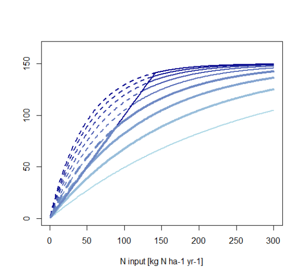
Figure 44: Crop growth curves according to Godard et al. (2008) for different crop growth scaling factors.
Figure 45: N input rates that give a yield of 80% of the maximum yield for different crop growth scaling factors according to Godard et al. (2008)
Lower efficiency for manure application
We assume that manure is applied with less efficiency than mineral fertilizer. First, because we take into account lower nutrient availability in manure with respect to mineral fertilizer (due to reduced opportunity to target release of nutrients to crop demand, thus increasing the chance of nutrient releases in periods with enhanced risks of losses to the environment). Second, due to the fact that higher availability of manure often goes ahead with increased lack of surface where the manure can be applied in a reasonable manner.
Therefore, we assume a decrease of the NUE the higher the share of manure in the fertilizer mix.
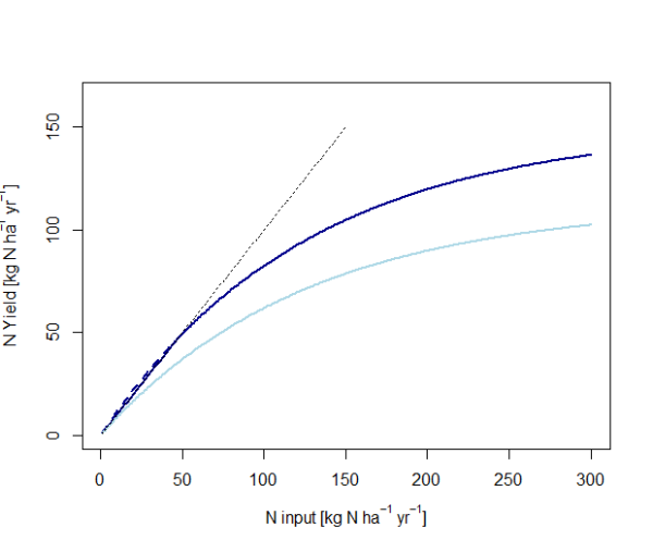
We account for this fact by using a different crop response curve for mineral fertilizer and manure. This is realized by varying the theoretical crop curve’s maximum yield.
This is shown in figure below.
Figure 46: Examples of crop response curves according to Godard et al. (2008).
We introduce a dependency of ymx on the share of mineral fertilizer and manure in the mix of the nitrogen source.
\begin{align} \begin{split} y_{h,c}^{mx} = y_{man,r,c}^{mx}+y_{man,h,c} \cdot (y_{min,r,c}^{mx}-y_{man,r,c}^{mx}) \\ χ_{man,h,c} = \frac {q_{man,h,c}} {q_{man,h,c}+ q_{min,h,c}} \end{split} \end{align}
\(y_{h,c}^{mx}\) = Maximum yield [variable, kg N ha-1 yr-1] according to the crop response curve (Godard et al., 2008) for crop c in the spatial unit h.
\(y_{man,r,c}^{mx}\) = Maximum yield for manure [parameter, kg N ha-1 yr-1] according to the crop response curve (Godard et al., 2008) for crop c in spatial unit h.
\(y_{min,r,c}^{mx}\) = Maximum yield for mineral fertilizer [parameter, kg N ha-1 yr-1] according to the crop response curve (Godard et al., 2008) for crop c in spatial unit h.
\(χ_{man,h,c}\) = Share of manure [variable, dimensionless] in the application of nitrogen from manure and mineral fertilizer.
Manure availability
Manure can be traded between individual spatial units. Manure trade between regions (or even countries) is covered by the regional model of CAPRI and does not need to be considered here.
The availability of manure is obtained therefore from each spatial unit plus neighboring spatial units within the same region. The range of spatial units from which manure can be used is assumed to a region-specific variable and
\begin{align} \begin{split} \sum_{c} \{ q_{man,h,c}\cdot a_{h,c} \} & \le \sum_{h^\prime,l} \{ e_{man,h,l}\cdot n_{h,l} \} \\ d_{h,h^\prime} & \le D_r^{mx} \end{split} \end{align}
\(q_{man,h,c}\) = Manure application rate [variable, kg N/ha] to crop c in spatial unit h
\(a_{h,c}\) = Area [parameter, 1000 ha] cultivated with crop c
\(e_{man,h,l}\) = Manure excretion [parameter, kg N/head] by animal species l in spatial unit h– net of losses in livestock housing and manure storage and management systems. No heterogeneity is assumed for nitrogen excretion rate within one NUTS2 region.
\(n_{h,l}\) = Livestock number [parameter, 1000 heads]
\(d_{h,h^\prime}\) = Distance [parameter, km] between spatial unit h and spatial unit h´
\(D_r^{mx}\) = Maximum distance [variable, km] for which transport of manure is allowed in region r.
Obviously, the total manure available for application must be exhausted:
\begin{equation} \sum_{h,c}\{q_{man,h,c}\cdot a_{h,c}\} = \sum_l \{ E_{man,r,l}\cdot N_{h,l} \} \end{equation}
Fertilization distribution model
Recover regional N flows
For each flow of nitrogen and crop, the sum of flows over all spatial units must recover the total flow at regional level for each crop.
This holds both for input flows and output flows (i.e. harvest, surplus).
Potential yield
The maximum (potential) yield is proportional to the relative potential yield (without water limitation).
\begin{equation} y_{h,c}^{mx} = F_{r,c}^{ymx}\cdot r_{h,c}^{py} \end{equation}
\(y_{h,c}^{mx}\) = Maximum yield [variable, kg/ha] determining the shape of the crop growth curve in each spatial unit for each crop.
\(r_{h,c}^{py}\) = Relative potential yield [parameter, dimensionless] of crop c in spatial unit h.
\(F_{r,c}^{ymx}\) = Scaling factor [variable, kg/ha] adjusting the relative potential yield so that it gives the maximum yield in the crop growth curve for each spatial unit h and crop c.
Crop growth curve
Total input of nitrogen is obtained from the observed yield for the crop in the spatial unit (parameter, calculated in the yield and irrigation module) and the maximum yield obtainable in the crop in the spatial unit (variable).
\begin{equation} q_{h,c} = -\frac{1}{x}\cdot ln \left\{ \frac{y_{h,c}}{y_{h,c}^{mx}} \right\} \end{equation}
Nitrogen source
Once the total N input per crop and spatial unit is determined, the individual N sources need to be calculated. We have:
- Biological N fixation: this is directly calculated from the crop type and yield and is ‘fixed’
- Atmospheric deposition: this is obtained from external data and cannot be modified
- Mineralization of soil organic matter. We have no data yet for calculating mineralization of soil organic matter at the regional level, thus it is not possible to include this term in the disaggregation. If there were data on soil organic mineralization, the following assumptions would need be taken:
- Mineralization of soil organic matter occurs in extensive fields, thus at low application rates of mineral fertilizer and irrigation rates
- Manure is able to replenish soil organic matter. It is thus unlikely that mineralization of soil organic matter occurs where manure is applied or deposited by grazing animals.
Data preparation
Collecting information
At Nuts2 level, y and f are known and ym can be calculated
\begin{equation} y_{r,c}^{mx} = \frac{y_{r,c}}{1-exp\{-f^{cropcurve}\cdot Q_{r,c}\}} \end{equation}
For each spatial unit, the yield is given from the distribution of irrigation shares and yield.
We can assume that the potential yield ym follows the pattern of the irrigated yield obtained from PESETA.
\begin{equation} y_{h,c}^{mx} \propto r_{h,c}^{py} \end{equation}
\(r_{h,c}^{py}\) = Relative potential yield [parameter, dimensionless] of crop c in spatial unit h.
Calculation of relative potential yield per spatial unit
\begin{equation} r_{h,c}^{py} = y_{h,c}^{py}/\overline{y_{h,c}^{py}} \end{equation}
\(r_{h,c}^{py}\) = Relative potential yield [parameter, dimensionless] of crop c in spatial unit h.
\(\overline{y_{h,c}^{py}}\) = Average potential yield [parameter, kg/ha] of crop c in region r.
\begin{equation} \overline{y_{h,c}^{py}} = \frac{\sum_h\{y_{h,c}^{py}\cdot a_{h,c}\}}{\sum_h\{a_{h,c}\}} \end{equation}
Calculation of distances between HSUs
Update pending
Calculation of manure availability
Excretion net of all volatilization must be back-calculated so that emissions from applications are not subtracted.
Update pending
Consideration of mitigation options
Update pending
Data Distribution Procedures
The terms spatial “resampling”, “re-mapping, “downscaling”, “disaggregation” and “distribution” are frequently used in a synonymous way. Admittedly, a very sharp distinction is sometimes difficult and there are overlaps in their meaning, this holds especially for “downscaling” and “disaggregation”. To avoid confusion of the reader we lay down our interpretation of these terms.
Resampling
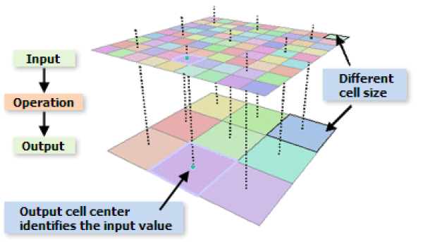
By resampling we intend the process of interpolating from one grid resolution to a different grid resolution. Quantitative evaluation of data contained on different grids requires resampling to a common grid. There are many resampling methods. Classic interpolation methods include: bilinear, nearest neighbor, inverse distance. The consistency with the original dataset is not necessarily maintained.
Example: Resampling of land use information at a regular grid of 100 x 100m from remote sensing to a 1km x 1km grid using the nearest neighbor method. The 1 x 1km grid receives the value of the 100 x 100 m grid which spatially coincides with the center of the 1 x 1km grid.
Re-mapping
In the context of this work we use the term re-mapping if the spatial reference unit of a given parameter has to be changed. The aim is to keep changes of the parameters/values at a minimum during the change of the spatial reference. Re-mapping is often required for pre- and post processing of data input/output of the downscaling/disaggregation/distribution procedures.
In the special case of nested data (i.e. a spatial unit at low hierarchical level is member of exactly one unit at a higher hierarchical level s. definition below) the re-mapping of values given at low hierarchical level to a higher hierarchical level can be obtained by simple aggregation (summing up or averaging). A typical example is the re-mapping of information given for administrative regions (NUTS3 - > NUTS2 → NUTS1 → NUTS0).
Definition of nested spatial reference data sets
\begin{equation} if \; 0 \lt a_{ij} \le 1 \; for\; i\in I \;and\; j\in J \; then\; a_{ik}=0 \;for \;i\in I \;and\; k\ne j \;and\; k\in J \end{equation}
More frequently data is stemming from various sources having different spatial reference units. For example meteo data which usually comes at a grid level (e.g. 50 x 50 km) and has to be re-mapped to an administrative unit. In these cases a spatial overlay of the data is performed and new spatial units are created at the intersection of the spatial units. In the meteo grid/administrative region case a meteo grid might be split by the border between 2 different administrative units.
To avoid creating very small spatial units during the re-mapping procedure we defined a minimum spatial unit of 1 x 1 km2 (i.e. the 1 by 1km EEA reference grid) as common denominator. All input data is rasterized or resampled to this unit before the re-mapping. For categorical data as e.g. land use/cover classes, the nearest neighbor interpolation method is applied. In other cases the share of the parameter in the 1 x 1 km2 grid is calculated (e.g forest area). After rasterizing/resampling of all data sets of interest, re-mapping of all parameters to any spatial reference unit present in the input data sets is possible.
Example: meteo data at 50 x 50 km grid level re-mapped to NUTS2 regions
Consistency of data between the rasterized versions of both spatial references is maintained:
\begin{equation} x_i=\frac{\sum_j x_j \cdot a_{ji}}{a_i} \end{equation}
I = units of the first layer (e.g. 50 km x 50 km grid)
J = units of the second layer (e.g. NUTS2 regions)
x = Area-based variable (e.g. average annual rainfall mm/m2; kg N/ha emissions; persons/ha; etc.)
a = Area. ai is the area of a unit of the layer the variable is re-mapped to. aij are the areas of the intersections between unit i and all units j that have common surface.
In case that \(\sum_j a_{ij} \le a_i\), that is there is a part of unit i which is not covered, assumptions on ‘gap-filling’ have to be made. Possible options are:
- Assuming same area-based variable thus giving higher total quantity
- Maintaining total quantity thus ‘diluting’ the area-based variable.
Increasing the spatial resolution of data for nested spatial references
We differentiate approaches for increasing the spatial resolution of data that are applicable to nested spatial data sets in view of the complexity of the approach. The complexity increases from simple distribution over downscaling to disaggregation.
Downscaling
As downscaling we understand a procedure to infer high-resolution information from low-resolution variables using simple proxy information that is available at the high resolution. Downscaling works only with nested spatial units. The consistency with the original dataset is maintained.
For example:
- downscaling population density in rural areas available at country level to a grid taking into account land cover information (rural areas/urban areas)
- downscaling of fertilizer input from national fertilizer use statistics based on distribution of crop yields available at higher spatial level (e.g. sub-national regions).
Disaggregation
Spatial disaggregation is the process by which information at a coarse spatial scale is translated to finer scales using weighting. The weights are based on more or less complex regression or other (optimization) models derived from observations, ancillary data, or previous downscaling/disaggregation steps. The consistency with the original dataset is maintained. One example is the use of LUCAS land use observations, environmental and management parameters to predict the probability of a crop to be cultivated at a certain location.
Simple Distribution
This procedure is applied if a parameter is available at high hierarchical level (e.g. country) and no information is available to enhance the spatial pattern for the lower hierarchical level (by proxies/regression/models) In this case, the spatial distribution of a parameter when changing the spatial reference unit from a higher to a lower hierarchical level is kept constant. Example: average nitrogen excretion rates for different livestock available at country level. A homogeneous distribution within all sub-units is assumed. Due to lacking information the effects of sub-national differences due to e.g. specific feeding strategies, are not taken into account.
