This task prepares and partially combines FAO data originally contained in separate tables from the FAOstat webpage to finally store them in gdx files for further use. This refers to: Commodity balances, production and landuse statistics (all stored in faodata.gdx), special balances for dairy products (fao_milkdata.gdx), population (fao_population.gdx), as well as the bilateral trade matirix (fao_trade_for_global.gdx).

The FAOSTAT task consists of two independent consolidation routines, the (A) Country data, and the (B) Trade flow related consolidation part. Part (A) imposes consistency rules on market balances, yields, activity levels, land use data, and population at the country level. Part (B) consolidates bilateral trade at the level of CAPRI trading blocks comprising quantities, values, unit values (UVAL) and the world price index (PRII).

The task requires input data stemming from an external preparation routine which is not a CAPRI module or sub-module. It is executed only on an intermittend basis depending on the availability of new raw data from FAOSTAT and the requirement for an update of the corresponding input data.

The resulting output from the external preparation routine are six gdx-files that have to be present in the \dat-folder of the CAPRI working directory: (1) commodityBalances, (2) population, (3) ProductionAndRessources, (4) fao_trade_matrix. Input data files (1) to (3) are required for the country related part (A), the trade matrix (4) is required for consolidation part (B).

In this step (1) activity levels, yields and production quantities are checked for completeness and heuristic rules are applied for gap filling. The (2) information on production statistics on crops is mapped to the commodity balances for the primary product equivalent to produce consistent data on yield and area. The (3) land use data is consolidated such that nested land categories add up to their totals. As the milk sector in FAOSTAT is organized differently from the CAPRI concept the (4) products’ mapping of the dairy sector is adjusted accordingly. (5) Gaps in population data for Serbia and Montenegro and for Belgium and Luxembourg are filled as well.

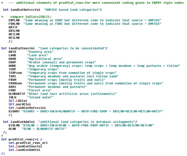
The head section of the sub-module comprises (a) initialization of FAOSTAT-related and mapping sets which are used in all futher consolidation sections, (b) loading union sets from the CommodityBalances and ProductionAndRessources data files, © introducing the land categories relevant for the land use consolidation, (d) introduction of multiplication factors for the mapping of units between FAOSTAT and CAPRI items, and (e) initialization of parameters. The © land categories relevant for the land use consolidation are as follows:

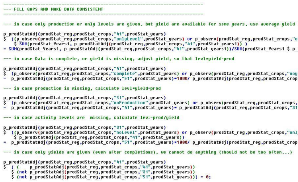
The first consolidation section is on “Production and Ressources”. After loading the raw data at the beginning, the FAOSTAT units are mapped to CAPRI units via the “unit_map” set and corresponding multiplication factors as provided under (d) in the head section of the program to harmonise the units. After that the data is checked for completeness and various heuristic rules are applied to fill gaps in the data:

After aggregating data for China and some reporting on missing data the consolidated production data is written to the \fao folder in the restart-directory for usage in the following consolidation steps.

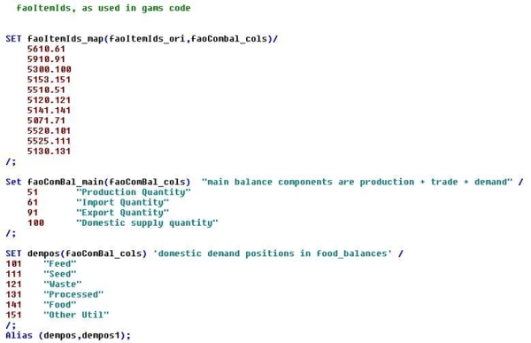
The next stept consolidates “Commodity Balances” and introduces the sets for the main balance components and demand positions as well as the mapping between the original FAOSTAT item codes and the commodity balance codes. This is another example that any data consolidation combining different data sets (even when coming from the same agency like FAO) needs to consider different coding systems used in those data sets:

In addition to the item code and unit matching and the removal of flags, negative observations are removed (except for stock changes) from the data. Gap filling is based on weighted averages and smoothed interpolation. Total demand is added up from single demand positions if missing and single demand positions are scaled to given total demand in case they do not sum up consistently. Finally, stock changes are adjusted to ensure that market balances are closed. The consolidated commodity balance data is written to the \fao-folder in the restart directory for further usage inside the fao_balance_consolidation.

The next stept combines production and ressources with the data on commodity balances in order to consolidate the land use data. The consolidation procedure for land use categories is a separate sub-routine included under this section:

The land use consolidation step takes care of the mapping between FAOSTAT and CAPRI land use categories, imposes gap filling routines, introduces auxiliary data from UNFCCC and UNSTATS and ensures that nested land use categories consistently sum up to their totals.

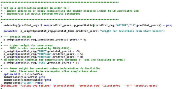
The land use consistency is solved as an optimization problem ensuring (a) adding up of single crop areas to land use aggegates and (b) imposes constraints stemming from transition probabilities between different UNFCCC land use categories:

Finally, crop area levels are rescaled based on the solution from the optimization problem and yields are recalculated accordingly. The consolidated land use data is written to the \fao-folder in the restart directory.

The next step consolidates data for the milk sector. The FAOSTAT market balances differ from CAPRI in four aspects that require special adjustment in addition to the mapping and gap filling routines. (1) Farm household production is not included in output from CAPRI COCO module but in the data from FAOSTAT, (2) Liquid whey and (3) liquid skimmed milk are considered in FAOSTAT but not in COCO, (4) Raw milk is not disaggregated into a category for final consumption as required by COCO. At the end of the consolidation section the result is written to \fao-folder in the results-directory. This file is also a major input for the CAPRI GLOBAL module (\fao\fao_milkdata_…gdx).

Data on population only requires adjustments for Serbia, Montenegro, and China which is taken care of in the following step. The aggregated population time series for Serbia and Montenegro from before 2006 is prolonged to the time after whereas the respective disaggregated time series are back-casted to the period before. Data for China is aggregated. The result is written to the \fao-folder in the results-directory which is a major input for the CAPRI task “Build global database”.

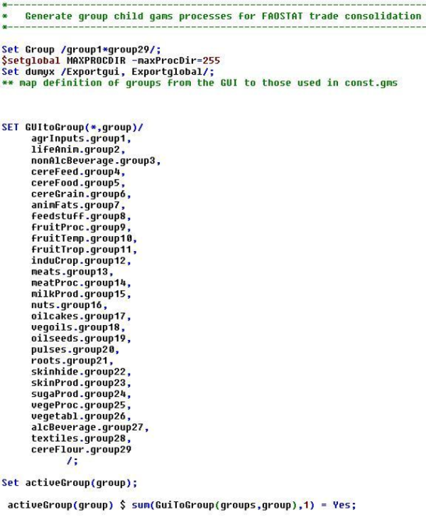
The consolidation of trade flows is split up across product specific groups to keep the task feasible in terms of computational complexity. The task is split up among 29 groups in total:

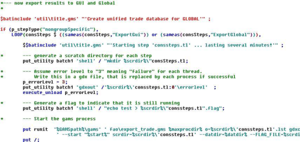
The whole procedure for creating a consistent data base as a starting point for the CAPRI task “Build global database” consists of two major tasks that are called the “groupSpecific” and “nongroupSpecific” tasks. The first one is the actual consolidation part that is done for each commodity group separately but executed in parallel. The second one is necessary for exporting the results such that they may be exploited via the GUI or be used as major input for the GLOBAL module.

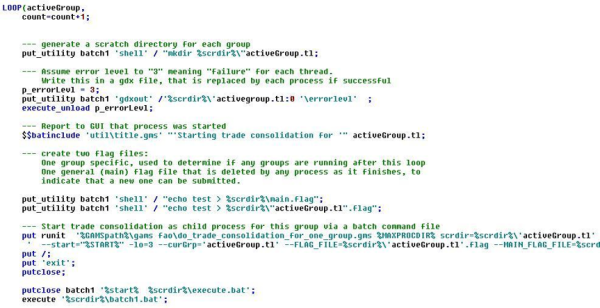
The group specific task starts 29 separate consolidation processes in parallel where the actual consolidation processes are defined in the separate include file “\fao\do_trade_consolidation_for_one_group.gms”.

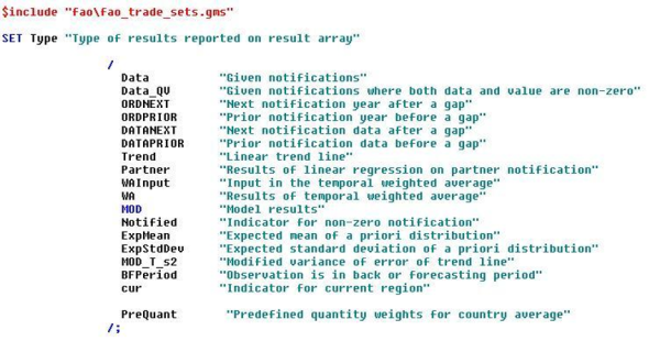
The trade consolidation part requires specific FAOSTAT trade data related sets that are loaded at the beginning of the include file. There are 18 different types of output reported in the result array.

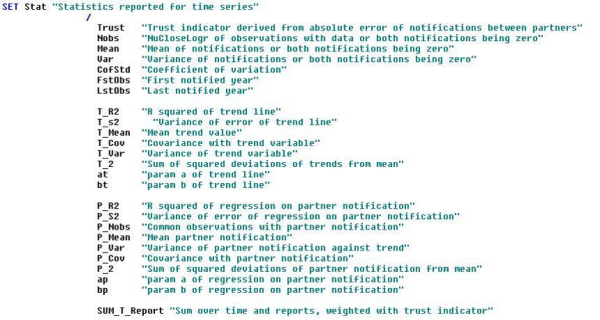
There are also 25 different statistics reported for the time series that are important intermediate indicators for the trade consolidation process.

The trade consolidation consists of eight steps in sequence that are dependent on each other, i.e. each step produces an intermediate output file that is written to the \fao folder in the restart directory for usage in the follow-up steps.

The process starts with the (1) SELECT step loading the raw trade data from the file “\dat\fao\FAO_trade_matrix_…gdx” which was produced by an external data preparation routine as described under the head section of this chapter. The raw data are just unloaded without any modifications in smaller files containing only the trade flows for one of the 29 product groups which facilitates subsequent processing. The next step is (2) AGGTRADE taking care of cutting off trade below a threshold of 1.E-5 and assigning a dummy variable for the case that trade was above this threshold.

The following step (3) UVATRADE filters trade flows computes unit values after some filtering procedures and fills gaps of their national times series based on linear interpolation. Time series of the producer price index are also completed based on averaging over different time horizons, on group averages, and on unit values.

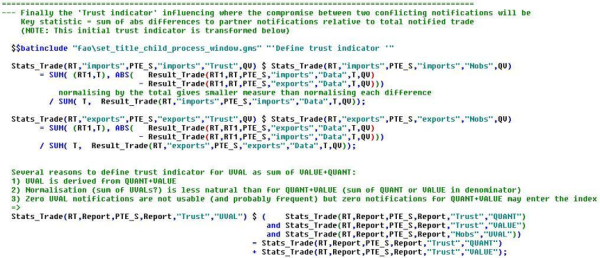
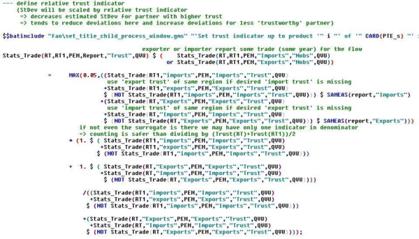
In the following step (4) STATRADE a trust indicator is computed that allows to assign a trade flow value in case of conflicting notifications between trade partners. It is based on the sum of absolute differences to partner notifications relative to total notified trade.

The next step (5) TRDTRADE calculates national linear trend lines for quantities, values, unit values and price indices.

Step (6) INITRADE prepares the trade data for the final consolidation procedure by calculating expected means of imports, exports and unit values, and by computing the trust indicator, standard errors and expected standard errors for trade quantity and units, and unit values. The trust indicator is used for adjusting the standard errors in the estimation of trade flows between partners. Higher trust indicators result in lower standard errors and lower standard errors lead to smaller deviations from reported trade, i.e. the outcome from the estimation will deviate less from the reportings for more trustworthy partners, and vice versa.

The computations are accomplished for each commodity separately.

Step (7) MODTRADE solves the trade consolidation problem by a Highest posterior density approach under constraints of (a) minimizing deviations from the expected means as computed in step (6), (b) minimizing dispersion around yearly country averages, © binding country level to world level unit values, and by (d) tying relative changes in country level unit values to relative changes in world unit values.

Finally, (8) SHOWTRADE stores the consolidated trade flow quantities in a gdx-file for exploitation and inspection.

The second “nongroupSpecific” task in the trade consolidation part takes care of exporting the consolidated trade data to the \fao-folder in the results directory. This output is a major input for the CAPRI task “Build global database” (“fao_trade_for_global…gdx”). The trade data is complemented with data on conversion coefficients, on extraction rates, mappings between product equivalent and product codes, and between raw and processed goods, production data on the animal sector, and caseinTrade. The export job is included as a separate program under the nongroupSpecific task.

The main program ¹⁾ for this task is capri\gams\global_database.gms which collects a number of included files for separate sub-tasks, some of which being trivial, others more complex.

Figure 9: Overview on key elements in the consolidation of global data (in global_database.gms)

Source: own illustration

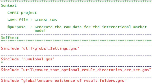
The program starts with including three general programs also present (possibly in task specific form) in other main programms plus the steering file (runglobal.gms) with more precise settings for the current run which may come from the GUI or from a batch file²⁾:

After these general settings the programm continues in a rather standard manner with a section collecting various declarations of sets and parameters. Among these are the general sets of CAPRI (sets.gms), and the sets specific to the market model (arm_sets.gms) because the purpose of the task is to compile the data needed for the market model at the global level of CAPRI:

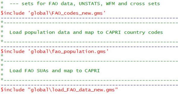
The most important data source for task “Build global database” is FAOstat which involves a fairly long file (FAO_codes_new.gms) with sets and cross-sets to map from FAO regions, items, and products into the CAPRI world (defined by the code system in the annex). This serves to map some key data from FAO compiled in the previous task: population (fao_population.gms), commodity balances combined with production and landuse statistics. Furthermore special balances for dairy products are loaded (all in load_fao_data_new.gms).

The second most important group of data, both historical as well as projections, for the global market model of CAPRI come from the Aglink-Cosimo model³⁾, including its ex post database.

• The first $include file (load_%aglink%_new.gms⁴⁾ ) includes the relevant sets to handle the Aglink data, including the cross-sets to map to CAPRI. In addition it also merges a special data set on fish markets with other original Aglink data.
• The next file (biofuel_markets.gms) data set builds biofuel market balances for non-EU regions, as FAOstat do not include biofuels and their demand for agricultural goods, but biofuel markets for EU countries are covered in COCO1 and the special projection tool for European regions (captrd.gms). This is an example for special treatments in the biofuel sector which are often unavoidable.
• The third $include file (growth_factor_aglink.gms) performs the first steps of data processing for the bulk of market balance data from Aglink-Cosimo: Items are mapped to the CAPRI codes, prices are converted from national currency into Euros, and projections from Aglink-Cosimo are converted into growth factors such that they may be conveniently combined with historical data from FAOstat (in “create_final_marketdb.gms).
• Finally the fourth file collects and maps various elasticities to the CAPRI coding system in order to serve as prior values in the CAPRI elasticity trimming code (trim_par, called during market calibration). Of these currently only the supply elasticities are used, such that this program gives a typical example of historicall grown coding: Obsolete elements are more often overwritten or ignored rather than deleted.

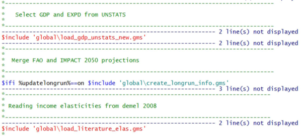
The next three $include files cover additional macroeconomic data from UNstats (load_gdp_unstats_new.gms), include and map long run projections beyond the Aglink horizon from the GLOBIOM⁵⁾ model (create_longrun_info.gms, comment “merge FAO and IMPACT 2050 projections is obsolete), and collect prior values for demand elasticities from the literature (collect_literature_elas.gms, whereas demand elasticties from Aglink-Cosimo are ignored).

It may be seen that “create_longrun_info.gms” is active or not depending on a setting from the GUI or a batch file. Similar to the code processing Aglink information it includes sets and mappings to handle the GLOBIOM information. Another similarity with the Aglink related files is that this code basically needs annual adjustments, because some definitions are changing from year to year and there are two GLOBIOM versions to distinguish, one with a certain EU focus, the other one with a perfectly global orientation. Finally, it may be mentioned that the projections are introduced into the CAPRI world mostly in the form of growth factors.

The CAPRI market model is spatial and therefore requires data on bilateral trade flows. These are covered in two include files, the first one dealing with the special case of biofuel trade flows, the second one with the general case.

Biofuel trade requires a special treatment again because FAOstat does not cover these. Instead, bilateral trade flows are constructed using total exports and imports from AGLINK and trade data from COMEXT, USDA and FO-Licht. By contrast the data for the trade matrix for other commodities is from FAOstat.

Both the biofuel trade matrix as well as non-biofuel trade are rendered “approximately” consistent with the totals from the previously collected market balance data with a small optimisation model that tries to minimise deviations from the prior data. File “map_tradeflow_to_capri.gms also tackles the problem of bilateral trade data entirely missing. In this case (relevant for fish, for example) default trade flows are introduced where commodities are mostly supplied by the largest exporters or imported by the most important importers.

After consolidating the trade flows two special data sets need to be considered. The first is a special data set on Switzerland checked in detail by the Swiss Federal Office on Agriculture (FOAG) and including trade flows involving Switzerland (hence included after the previous consolidation such that these data overwrite the trade flow information but also the market balance information from FAOstat).

The second is a transport cost matrix estimation using the original FAOstat trade matrix (so before gap filling and consolidation) and distance related information from CEPII. Together with price information the transport costs are estimated to provide a link between CIF and FOB prices for bilateral tradeflows.

The next $include file extends the Aglink-Cosimo projections to 2030, if needed, with a trend estimation involving a number of pragmatic modifications (such as the trend line passing trough the last observation). Then the the growth factors computed previously or the default trends are used to estimate a medium term outlook projections for global market balances, prices or GDP. These projections do however not include any consictency checks on closed market balances or similar properties. This is achieved in the baseline calibration only.

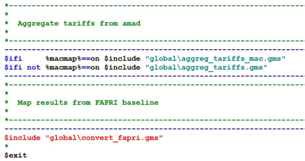
Finally, data on trade policy variables such as applied and scheduled tariffs, tariff rate quotas or bilateral trade agreements are collected from the Agricultural Market Access Database (AMAD, obsolete current version) or from the MacMaps database (%macMap%)⁶⁾==on, but not yet activated under Star2.4).

The very last include file is probably also the least important one: FAPRI projections had a more important role several years ago, are not updated anymore and presumable affect less than a dozen numbers (if any at all) in the global database compiled in this task: