CAPRI Online Manual (update)

Nitrogen input to fields needs to be distributed over the spatial units in a region where the crop is cultivated. For each crop, the regional nitrogen balance is given with total N inputs per N input type, an N outputs or losses per output and loss type.

We base the distribution model on a generic crop-fertilizer-response curve. Such curves have the characteristics that are desirable for the disaggregation of nitrogen input:

1. higher N input leads to higher yields;
2. with increasing levels of N input the yield increment decreases;
3. the N ‘uptake’ is always less of N input;
4. saturation, i.e. attaining about 80-90% of the maximum yield at about 100-200 kg N ha^-1 yr^-1

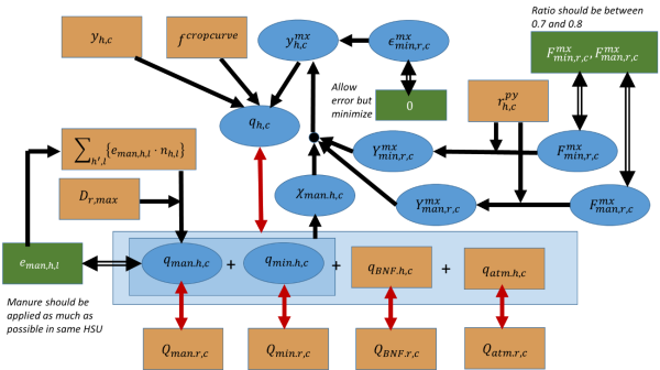
Such crop response curves ‘work’ with a maximum yield which are approached at high levels of N input. These maximum yield values are unknown. Figure below gives an overview of the approach indicating parameters, variables, and optimization rules.

Figure 43: Schematic overview of the Nitrogen disaggregation model

Source: own illustration

Different crop response curves are proposed (Bodirsky and Müller, 2014; Godard et al., 2008). We base our response curve on the proposal of (Godard et al., 2008) in particular for the ‘saturation’ velocity¹⁾.

\begin{align} \begin{split} &\text{Crop growth model (Godard et al., 2008)} \\ &Y_{r,c} = Y_{r,c}^{mx}-(Y_{r,c}^{mx}-Y_{r,c}^{mn}) \cdot exp\{-f^{cropcurve}\cdot Q_{r,c}\} \end{split} \end{align}

\begin{align} \begin{split} &\text{Crop growth model (Godard et al., 2008) without ‘minimum yield’} \\ &Y_{r,c} = Y_{r,c}^{mx}-(1 - exp\{-f^{cropcurve}\cdot Q_{r,c}\}) \cdot @ Y_{r,c}^{mn} = 0 \end{split} \end{align}

\(Y_{r,c}\) = Yield [parameter, kg N ha^-1 yr^-1] for crop c in region r.
\(Y_{r,c}^{mx}\) = Maximum yield [parameter, kg N ha^-1 yr^-1] according to the crop response curve (Godard et al., 2008) for crop c in region r.
\(Y_{r,c}^{mn}\) = Minimum yield [parameter, kg N ha^-1 yr^-1] according to the crop response curve (Godard et al., 2008) for crop c in region r. This parameter is set to zero in our model.
\(f^{cropcurve}\) = Scaling factor [parameter, dimensionless] used in the crop response curve (Godard et al., 2008). We use a uniform value of \(f^{cropcurve}=0.008\).
\(Q_{r,c}\) = Total N input [parameter, kg N ha^-1 yr^-1] for region r and crop c.

We use a constant factor \(f^{cropcurve}\) for all regions/spatial units and crops in order to not leave too many degrees of freedom. However, if infeasibilities occur, ‘opening’ this factor to differ between crop types could be a first test. However, the range of possible values for the crop growth scaling factor is narrow:

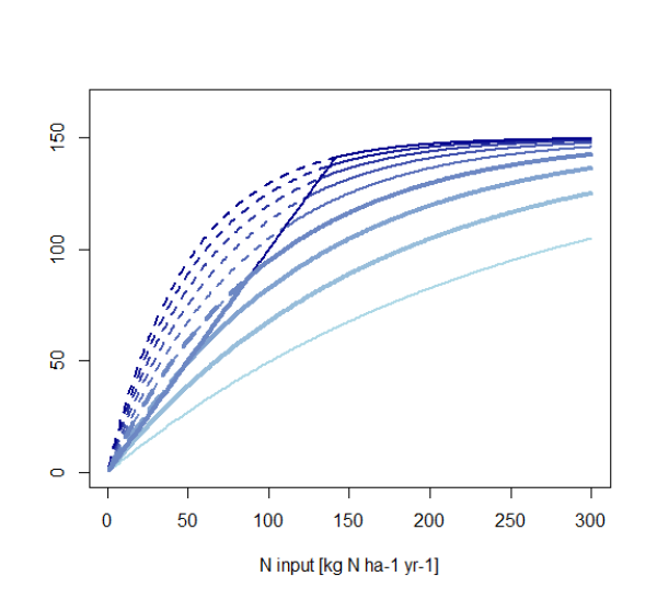
• For \(f^{cropcurve}>0.010\) a N uptake is larger than N input until an application rate of more than 100 kg N ha^-1 yr^-1. For a value of 0.010 this is the case for an application rate of about 100 kg N ha^-1 yr^-1
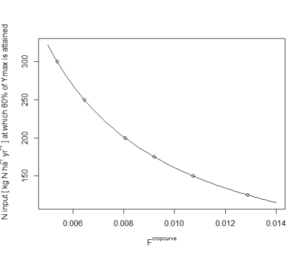
• For \(f^{cropcurve}<0.008\) the N input rate at which a yield of 80% of the maximum yield is attained is very high. For a value of 0.0064 this happens at Q=250 kg N ha^-1 yr^-1; and for a value of 0.0054 at Q=300 kg N ha^-1 yr^-1.

Therefore, only a narrow range around a value of 0.008 seems plausible.

Figure 44: Crop growth curves according to Godard et al. (2008) for different crop growth scaling factors.

Parameters from light blue to dark blue curves: \(0.004\le f^{cropcurve}\le 0.020\). The curves with \(f^{cropcurve} \in {0.006,0.008,0.010} \) are plotted in bold. Other parameter: Y^mx=150; Y^mn=0.

Figure 45: N input rates that give a yield of 80% of the maximum yield for different crop growth scaling factors according to Godard et al. (2008)

Lower efficiency for manure application

We assume that manure is applied with less efficiency than mineral fertilizer. First, because we take into account lower nutrient availability in manure with respect to mineral fertilizer (due to reduced opportunity to target release of nutrients to crop demand, thus increasing the chance of nutrient releases in periods with enhanced risks of losses to the environment). Second, due to the fact that higher availability of manure often goes ahead with increased lack of surface where the manure can be applied in a reasonable manner.

Therefore, we assume a decrease of the NUE the higher the share of manure in the fertilizer mix.

We account for this fact by using a different crop response curve for mineral fertilizer and manure. This is realized by varying the theoretical crop curve’s maximum yield.

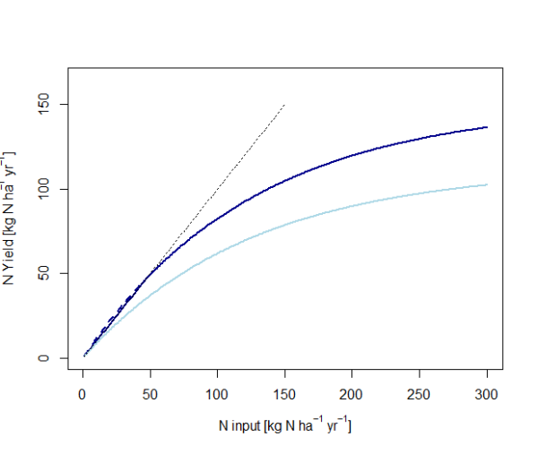
This is shown in figure below.

Figure 46: Examples of crop response curves according to Godard et al. (2008).

Parameters used: f=0.008. Light blue curve for manure: y^mx=130; dark blue curve for mineral fertilizer: y^mx=150.

We introduce a dependency of y^mx on the share of mineral fertilizer and manure in the mix of the nitrogen source.

\begin{align} \begin{split} y_{h,c}^{mx} = y_{man,r,c}^{mx}+y_{man,h,c} \cdot (y_{min,r,c}^{mx}-y_{man,r,c}^{mx}) \\ χ_{man,h,c} = \frac {q_{man,h,c}} {q_{man,h,c}+ q_{min,h,c}} \end{split} \end{align}

\(y_{h,c}^{mx}\) = Maximum yield [variable, kg N ha^-1 yr^-1] according to the crop response curve (Godard et al., 2008) for crop c in the spatial unit h.
\(y_{man,r,c}^{mx}\) = Maximum yield for manure [parameter, kg N ha^-1 yr^-1] according to the crop response curve (Godard et al., 2008) for crop c in spatial unit h.
\(y_{min,r,c}^{mx}\) = Maximum yield for mineral fertilizer [parameter, kg N ha^-1 yr^-1] according to the crop response curve (Godard et al., 2008) for crop c in spatial unit h.
\(χ_{man,h,c}\) = Share of manure [variable, dimensionless] in the application of nitrogen from manure and mineral fertilizer.

Manure can be traded between individual spatial units. Manure trade between regions (or even countries) is covered by the regional model of CAPRI and does not need to be considered here.

The availability of manure is obtained therefore from each spatial unit plus neighboring spatial units within the same region. The range of spatial units from which manure can be used is assumed to a region-specific variable and

\begin{align} \begin{split} \sum_{c} \{ q_{man,h,c}\cdot a_{h,c} \} & \le \sum_{h^\prime,l} \{ e_{man,h,l}\cdot n_{h,l} \} \\ d_{h,h^\prime} & \le D_r^{mx} \end{split} \end{align}

\(q_{man,h,c}\) = Manure application rate [variable, kg N/ha] to crop c in spatial unit h
\(a_{h,c}\) = Area [parameter, 1000 ha] cultivated with crop c
\(e_{man,h,l}\) = Manure excretion [parameter, kg N/head] by animal species l in spatial unit h– net of losses in livestock housing and manure storage and management systems. No heterogeneity is assumed for nitrogen excretion rate within one NUTS2 region.
\(n_{h,l}\) = Livestock number [parameter, 1000 heads]
\(d_{h,h^\prime}\) = Distance [parameter, km] between spatial unit h and spatial unit h^´
\(D_r^{mx}\) = Maximum distance [variable, km] for which transport of manure is allowed in region r.

Obviously, the total manure available for application must be exhausted:

\begin{equation} \sum_{h,c}\{q_{man,h,c}\cdot a_{h,c}\} = \sum_l \{ E_{man,r,l}\cdot N_{h,l} \} \end{equation}

For each flow of nitrogen and crop, the sum of flows over all spatial units must recover the total flow at regional level for each crop.

This holds both for input flows and output flows (i.e. harvest, surplus).

The maximum (potential) yield is proportional to the relative potential yield (without water limitation).

\begin{equation} y_{h,c}^{mx} = F_{r,c}^{ymx}\cdot r_{h,c}^{py} \end{equation}

\(y_{h,c}^{mx}\) = Maximum yield [variable, kg/ha] determining the shape of the crop growth curve in each spatial unit for each crop.
\(r_{h,c}^{py}\) = Relative potential yield [parameter, dimensionless] of crop c in spatial unit h.
\(F_{r,c}^{ymx}\) = Scaling factor [variable, kg/ha] adjusting the relative potential yield so that it gives the maximum yield in the crop growth curve for each spatial unit h and crop c.

Total input of nitrogen is obtained from the observed yield for the crop in the spatial unit (parameter, calculated in the yield and irrigation module) and the maximum yield obtainable in the crop in the spatial unit (variable).

\begin{equation} q_{h,c} = -\frac{1}{x}\cdot ln \left\{ \frac{y_{h,c}}{y_{h,c}^{mx}} \right\} \end{equation}

Once the total N input per crop and spatial unit is determined, the individual N sources need to be calculated. We have:

• Biological N fixation: this is directly calculated from the crop type and yield and is ‘fixed’
• Atmospheric deposition: this is obtained from external data and cannot be modified
• Mineralization of soil organic matter. We have no data yet for calculating mineralization of soil organic matter at the regional level, thus it is not possible to include this term in the disaggregation. If there were data on soil organic mineralization, the following assumptions would need be taken:
  • Mineralization of soil organic matter occurs in extensive fields, thus at low application rates of mineral fertilizer and irrigation rates
  • Manure is able to replenish soil organic matter. It is thus unlikely that mineralization of soil organic matter occurs where manure is applied or deposited by grazing animals.

At Nuts2 level, y and f are known and y_m can be calculated

\begin{equation} y_{r,c}^{mx} = \frac{y_{r,c}}{1-exp\{-f^{cropcurve}\cdot Q_{r,c}\}} \end{equation}

For each spatial unit, the yield is given from the distribution of irrigation shares and yield.

We can assume that the potential yield y_m follows the pattern of the irrigated yield obtained from PESETA.

\begin{equation} y_{h,c}^{mx} \propto r_{h,c}^{py} \end{equation}

\(r_{h,c}^{py}\) = Relative potential yield [parameter, dimensionless] of crop c in spatial unit h.

\begin{equation} r_{h,p}^{py} = y_{h,p}^{py}/\overline{y_{h,p}^{py}} \end{equation}

\(r_{h,c}^{py}\) = Relative potential yield [parameter, dimensionless] of crop c in spatial unit h.
\(\overline{y_{h,p}^{py}}\) = Average potential yield [parameter, kg/ha] of crop c in region r.

\begin{equation} \overline{y_{h,c}^{py}} = \frac{\sum_h\{y_{h,c}^{py}\cdot a_{h,c}\}}{\sum_h\{a_{h,c}\}} \end{equation}

Update pending

Excretion net of all volatilization must be back-calculated so that emissions from applications are not subtracted.

Update pending

Update pending